Sparse Planning in Visual World Models
via Cost Gradients

Goal-conditioned token selection for faster world-model planning, without retraining.

Yingchen XuEdward Grefenstette

NeurIPS 2026

Read paper Code forthcoming

01 / IN ACTION

Keep what matters for the goal.

PointMaze trajectory with retained visual tokens highlighted and discarded tokens dimmed — PointMazeNAVIGATION

Wall navigation trajectory showing the changing COSTGRAD token selection — WallNAVIGATION

PushT trajectory showing selected tokens around the pusher and T-shaped object — PushTMANIPULATION

MetaWorld reach trajectory showing selected tokens around the robot arm and workspace — MetaWorldREACH

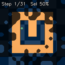
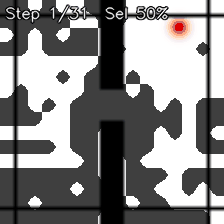
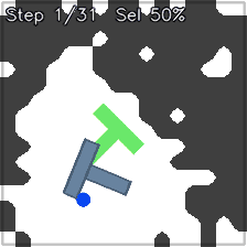
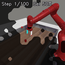
Bright: retained tokens Dim: discarded tokens

Recorded rollouts · 50% tokens · retrained predictors

128/256

spatial tokens per sparse rollout

2.6×

estimated planning-time speedup

gradient probe per planning step

02 / THE IDEA

Ask the planning objective.

Prediction and control need
different things from an image.

COSTGRAD scores each visual token by how strongly it affects the planning cost. A single gradient probe chooses the tokens; the planner then searches over actions using that smaller representation. The predictor stays fixed: no retraining is required.

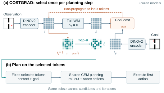
A full-token zero-action world-model probe produces a goal cost. Backpropagating that cost scores input tokens; top-K selection fixes the context and goal subset for sparse CEM planning and action execution. — Select once per planning step, then reuse the subset throughout action search. Reselect at the next observation. Token grids are schematic.

03 / PERFORMANCE

Less rollout compute.
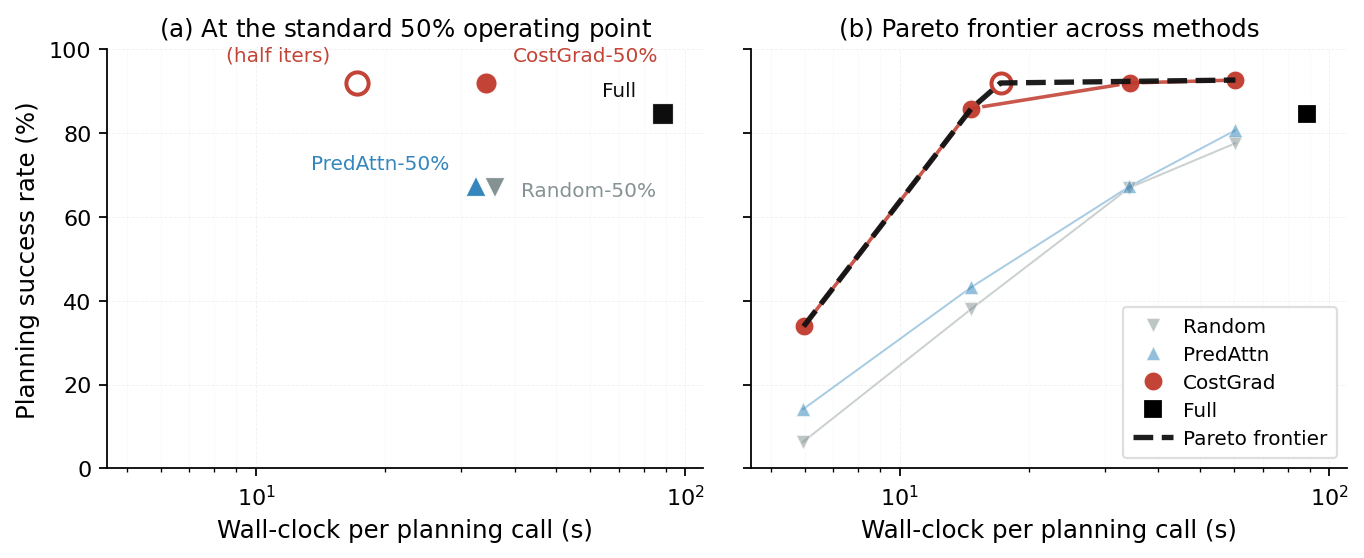
Strong planning performance.

50% TOKEN RETENTION

On the evaluated retrained AdaLN predictors, COSTGRAD achieves higher mean success than Full on three of four environments.

Retrained AdaLN checkpoints: mean planning success (%).
Environment	Full 256 tokens	COSTGRAD 128 tokens	Random 128 tokens	CG − Full percentage points
PointMaze	88.2	86.2	77.0	−2.0
Wall	84.7	92.0	67.0	+7.3
PushT	62.4	65.2	41.3	+2.8
MetaWorld reach	58.7	65.6	46.9	+6.9

Means across three runs per method and environment, with 96 episodes per run. These predictors are separate from the released-checkpoint control below.

Released JEPA-WMs checkpoints · no retraining

COSTGRAD also applies directly to released predictors. Full, COSTGRAD, and Random use the same checkpoint within each environment.

Released checkpoints: planning success (%), mean ± standard deviation over three evaluation seeds.
Environment	Full 256 tokens	COSTGRAD 128 tokens	Random 128 tokens
PointMaze	87.7 ± 7.7	86.3 ± 11.9	70.7 ± 15.1
Wall	87.0 ± 2.8	87.0 ± 2.2	75.7 ± 4.6
PushT	66.3 ± 2.6	67.3 ± 3.4	21.0 ± 9.0
MetaWorld reach	58.3 ± 10.0	63.2 ± 5.2	20.8 ± 9.0

96 episodes per evaluation seed. COSTGRAD and Random retain 50% of the tokens. The MetaWorld task is Reach.

Wall benchmark: planning success versus estimated planning time. At 50% tokens, fewer CEM iterations further reduce planning time. — **Token selection and search budget are complementary.** Component timings on the Wall predictor estimate a 2.6× planning-step speedup at 50% tokens, including selection overhead. Combining token selection with 15 rather than 30 CEM iterations gives an estimated 5.2× speedup.Times are reconstructed from encoder, selection, and predictor timings; they exclude CEM sampling/refitting and goal-cost evaluation.

04 / UNDERSTANDING SPARSE PLANNING

Token choice changes
the planning problem.

A token can matter for planning through its own prediction or by supplying context for predictions elsewhere. COSTGRAD uses sensitivity to the goal-reaching cost to identify that influence.

Removing tokens also changes the predictor’s computation. Sparse planning therefore depends on both the selected state information and the resulting action-conditioned rollouts.

Read the scope and limitations

Two effects of token removal

Which positions enter the cost: The planner compares predictions with the goal at retained positions.
What the predictor produces: Removing context can change predictions at those same retained positions.

Both effects can change how candidate actions are ranked.

Scope and future work

The performance comparisons above use AdaLN-conditioned predictors, DINOv2 visual features, CEM planning, and four simulated continuous-control tasks. Generality across other conditioning mechanisms, including FiLM and cross-attention, and evaluation on physical systems remain future work.

The displayed MetaWorld demo uses our retrained Reach predictor. The released-checkpoint control also evaluates Reach, using the public checkpoint. The one-step gradient probe selects tokens; action search still evaluates full-horizon rollouts.

05 / REFERENCE

Cite this work.

@inproceedings{xu2026sparseplanning,
  title     = {Sparse Planning in Visual World Models
               via Cost Gradients},
  author    = {Xu, Yingchen and Grefenstette, Edward},
  booktitle = {Advances in Neural Information Processing Systems},
  year      = {2026},
  url       = {https://arxiv.org/abs/2610.10274v1}
}

Sparse Planning in Visual World Modelsvia Cost Gradients